


 402 / 762

402
Chapter 9: The Normal Probability Distribution
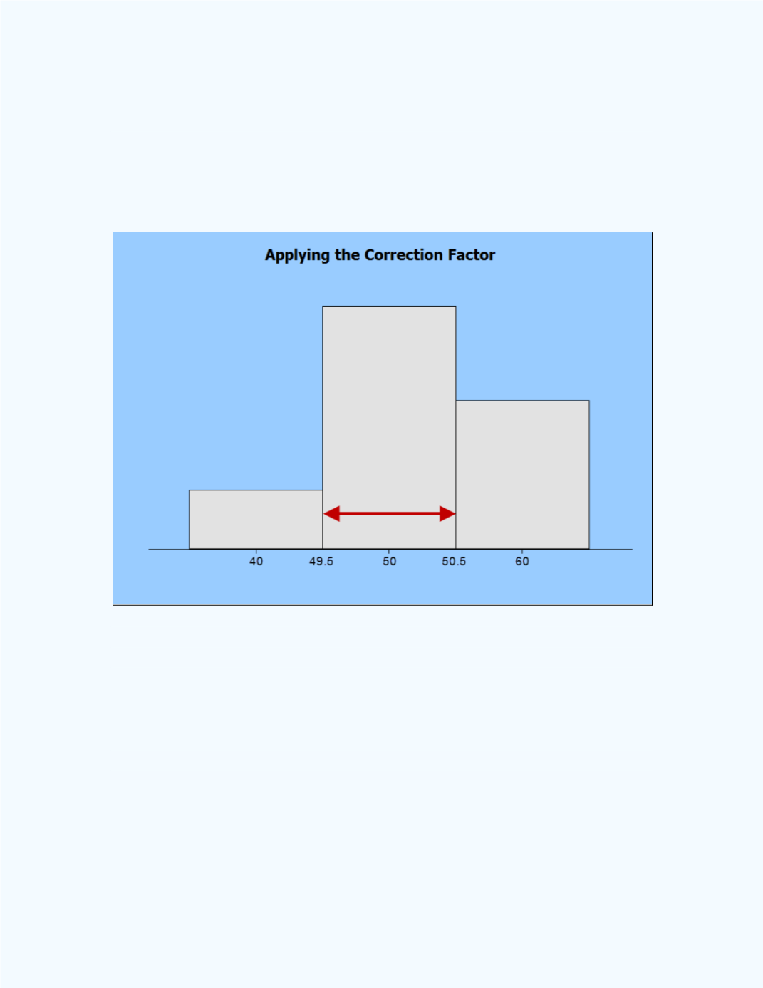
Thus applying the correction factor gives the following equivalence:
P
(
X
= 50)
P
(49.5
X
50.5).
Figure 9-38
shows how you will apply the correction factor for all possible
scenarios for a value of 50. Note that the center point of the bar of the
histogram represents where the discrete value of 50 is located.
Figure 9-38:
P
(
X
= 50) =
P
(49.5
X
50.5)
Case 2: P(X
a
) where
a
is the value of a Binomial random
variable X
If we needed to find P(
X
50) when
X
is a binomial random variable then
we will have to apply the continuity correction factor in order to use the
normal approximation since
X
is discrete. Since
X
= 50 is included
in
X
50, then we have to move 0.5 to the left of 50 to compute the
probability
P
(
X
50), in order to include the value of 50 in the computation.
Thus applying the correction factor gives the following equivalence:
P
(
X
50) ≡
P(X
49.5).