


 403 / 762

Chapter 9: The Normal Probability Distribution
403
Figure 9-39
shows how you will apply the correction factor in this case.
Note that the center point of the bar of the histogram represents where the
discrete value of 50 is located.
Figure 9-39:
P
(
X
50) =
P
(
X
49.5)
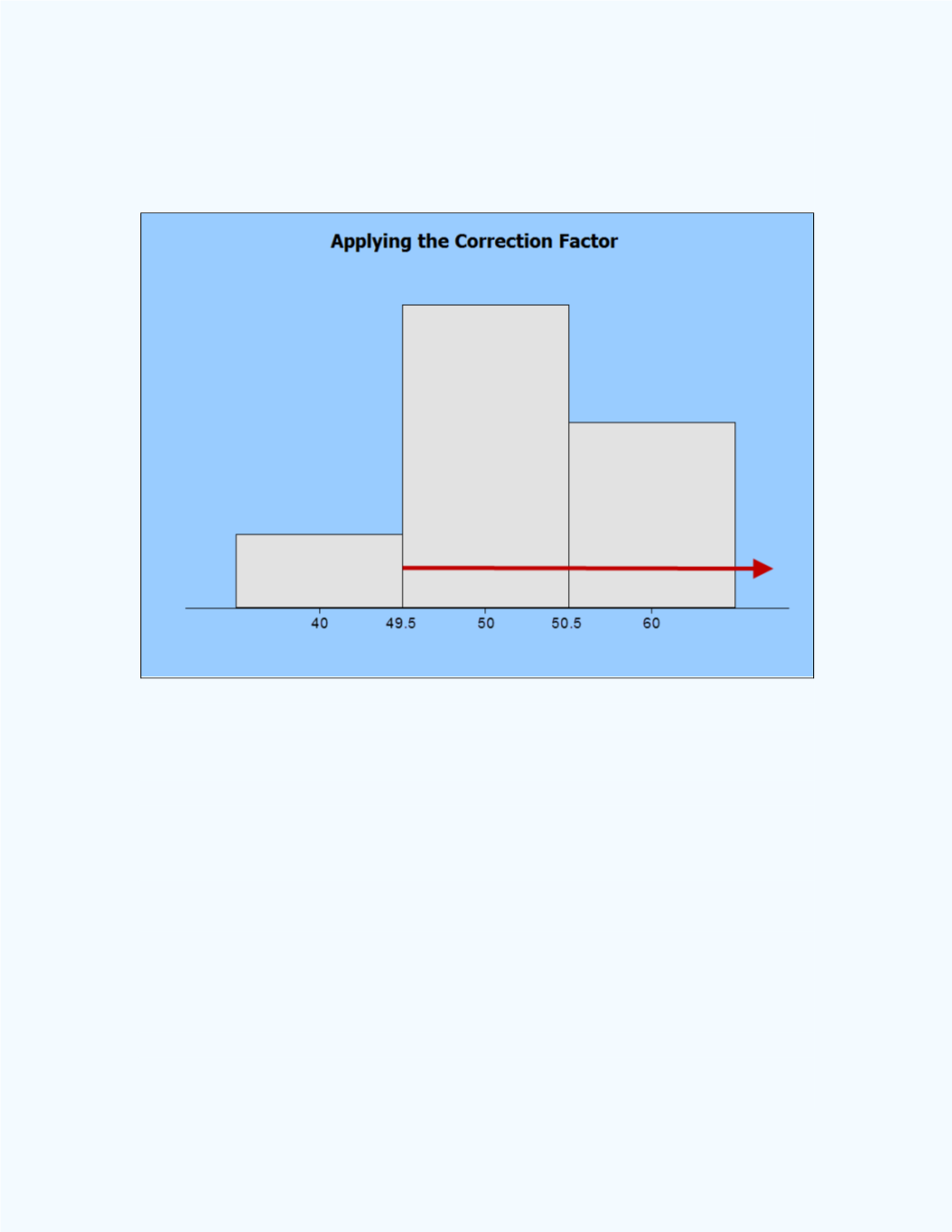
Case 3: P(X >
a
) where
a
is the value of a Binomial random
variable X
If we needed to find P(
X
> 50) when
X
is a binomial random variable then
we will have to apply the continuity correction factor in order to use the
normal approximation since
X
is discrete. Since
X
= 50 is not included in
X
> 50, then we have to move 0.5 to the right of 50 to compute the
probability
P
(
X
> 50), in order to not include the value of 50 in the
computation. Thus applying the correction factor gives the following
equivalence:
P
(
X
> 50)
P(X
50.5).
Figure 9-40
shows how you will apply the correction factor in this case.
Note that the center point of the bar of the histogram represents where the
discrete value of 50 is located.