


 141 / 762

Chapter 3: Measures of Variability
141
There are several formulas which one can use to compute the skewness for a
distribution of numerical values. Here we will discuss two formulas which
we can use to quantify this skewness property for a distribution. The
simplest, developed by Karl Pearson, one of the great contributors to the
science of statistics, is based on a relationship between the mean, median,
and the standard deviation. This measure is often called the
Pearson’s
coefficient of skewness
.
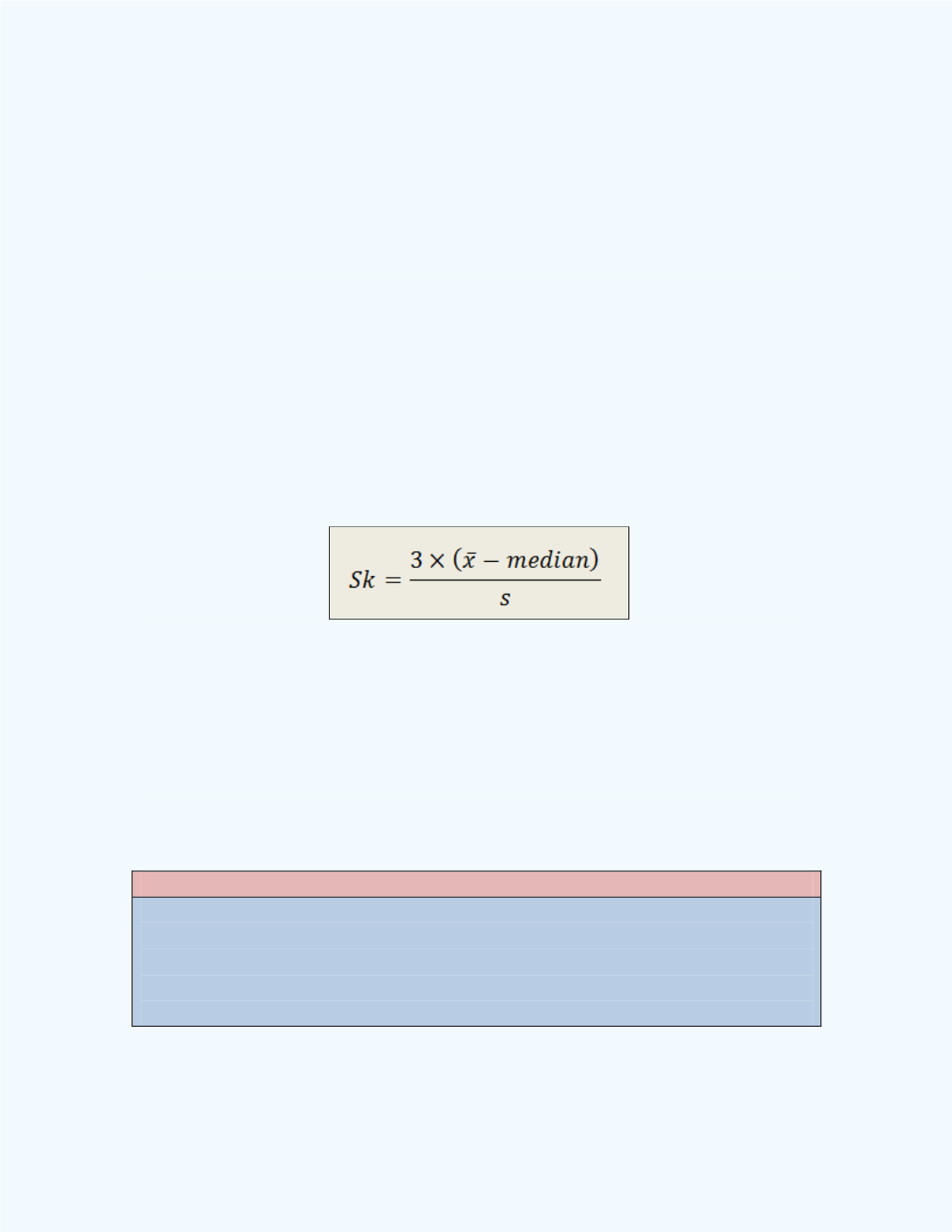
Pearson’s Coefficient of Skewness
The sample Pearson’s coefficient of skewness, denoted by
, is computed
from the following formula.
Example 3-15:
The information for a data set are as follows: mean = 10,
median = 8, and standard deviation = 4. Compute the Pearson’s coefficient
of skewness.
Solution:
Based on the information given,
= 3(10 – 8)/4 = 1.5.
Observe that this value is positive. Hence the distribution of values will
display a longer tail to the right.
Notes:
The Pearson’s coefficient of skewness can range from -3 to +3.
Pearson also developed the formula to compute the coefficient of
variation.