


 142 / 762

142
Chapter 3: Measures of Variability
Example 3-16:
Data was simulated and the following information was
obtained from the data: Sample Mean = 4.908, Sample Median = 3.419,
Sample Standard Deviation = 4.755. Compute the Pearson’s coefficient of
skewness.
Solution:
= 3(4.908 – 3.419)/4.755 = 0.9394
0.94.
Observe that the skewness is positive.
Note:
If we have data, we can use the Basic Statistics workbook to help
with the computations.
Example 3-17:
Find the Pearson’s coefficient of skewness for the
frequency counts for the chest size data given in
Section 3-7
.
Solution:
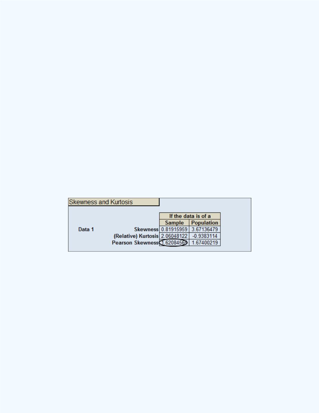
Since we have data, we can use the Basic Statistics workbook to
help with the computations.
Figure 3-32
shows the results when the
frequency counts were place in the Data 1 column.
Figure 3-32:
Pearson’s Skewness for
Example 3-17
The value turns out to be
= 1.6209 (to four decimal places). This value
reveals that the distribution will be somewhat skewed to the right.
Figure
3-19
reveals that the distribution is indeed skewed to the right.
The other formula used to compute the sample skewness is usually referred
to as the “software formula” because it is used in several software packages.