


 605 / 762

Chapter 13: Confidence Intervals – Small Samples
605
use the (after - before) weight differences. Thus, we will use the differences
(after - before) as the raw data in constructing the confidence interval.
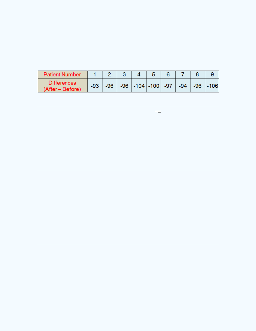
The (after – before) differences are given in
Table 13-5
.
Table 13-5:
The Differences of (After – Before) Weights
For the differences we have,
̅
= - 98,
= 4.4441,
n
= 9. Also,
= 0.05,
/2 = 0.025,
df
= 9 – 1 = 8,
= 2.3060, and
√
= 1.4814.
Thus, using the formula, the 95% confidence interval for the differences will
be -98
2.306
1.4814 or -98
3.4161.
That is, the dietician will be 95% confident that the average weight loss will
be between -101.4161 and -94.5839 based on the confidence interval using
the sample.
Observe that both end points of the interval are negative. This would
indicate that the average for the weights after the diet will be smaller than
the average of the weights before the diet. Thus, one may infer that the diet
seemed to be effective in the loss of weight.
Note, we can also use the
Small Sample Confidence Interval for The
Difference between Two Dependent Means
workbook to solve the
problem. We may use both the summary information and the differences
data in the workbook.
Figure 13-12
shows the output when the summary information is used to
construct the confidence interval. From
Figure 13-12
, the computed 95%
confidence interval is (-101.4260, -94.5840) to four decimal places. This
interval is slightly different from when the formula was used. The values
are off by 0.0001.