


 124 / 762

124
Chapter 3: Measures of Variability
Example 3-12:
Different brokers charge different amounts of fees to
manage an investment portfolio. An investor shopped around to get an idea
of the fees which will be incurred to manage two portfolios of stocks. He
found that the average monthly fee for (Portfolio A) was $275.00 with a
standard deviation of $65.257. Another portfolio of stocks (Portfolio B) had
an average monthly fee of $50.125 with a standard deviation of $15.525.
Compare the variations of the fees for the two portfolios. Assume the
portfolios of stocks represent the samples.
Solution:
(portfolio A) =
%73.23 %100
275
257 .65
(portfolio B) =
%97.30 %100
125 .50
525 .15
Since the
is larger for Portfolio B, then one could infer that there is more
variability in the fees charged by different brokers to manage Portfolio B.
Next we will discuss the population coefficient of variation.
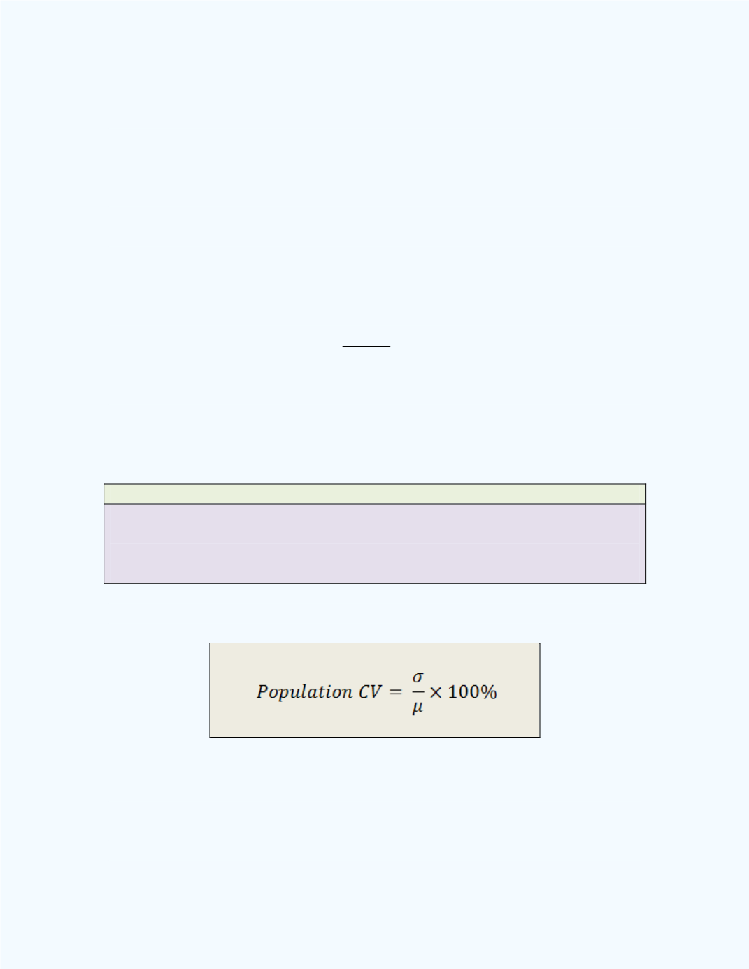
Definition: Population Coefficient of Variation
The population coefficient of variation is defined as the population standard
deviation divided by the population mean of the data set.
The formula used to compute this parameter is given next.
Note:
The population
has the same properties as the sample
. That is,
the population coefficient of variation standardizes the variation of the data
set by dividing it by the population mean. Thus the coefficient of variation
has no units, and so we can use this measure to compare variations for
different population variables with different units.