


 363 / 762

Chapter 9: The Normal Probability Distribution
363
Section Review
9 - 3 Properties of the Normal Distribution
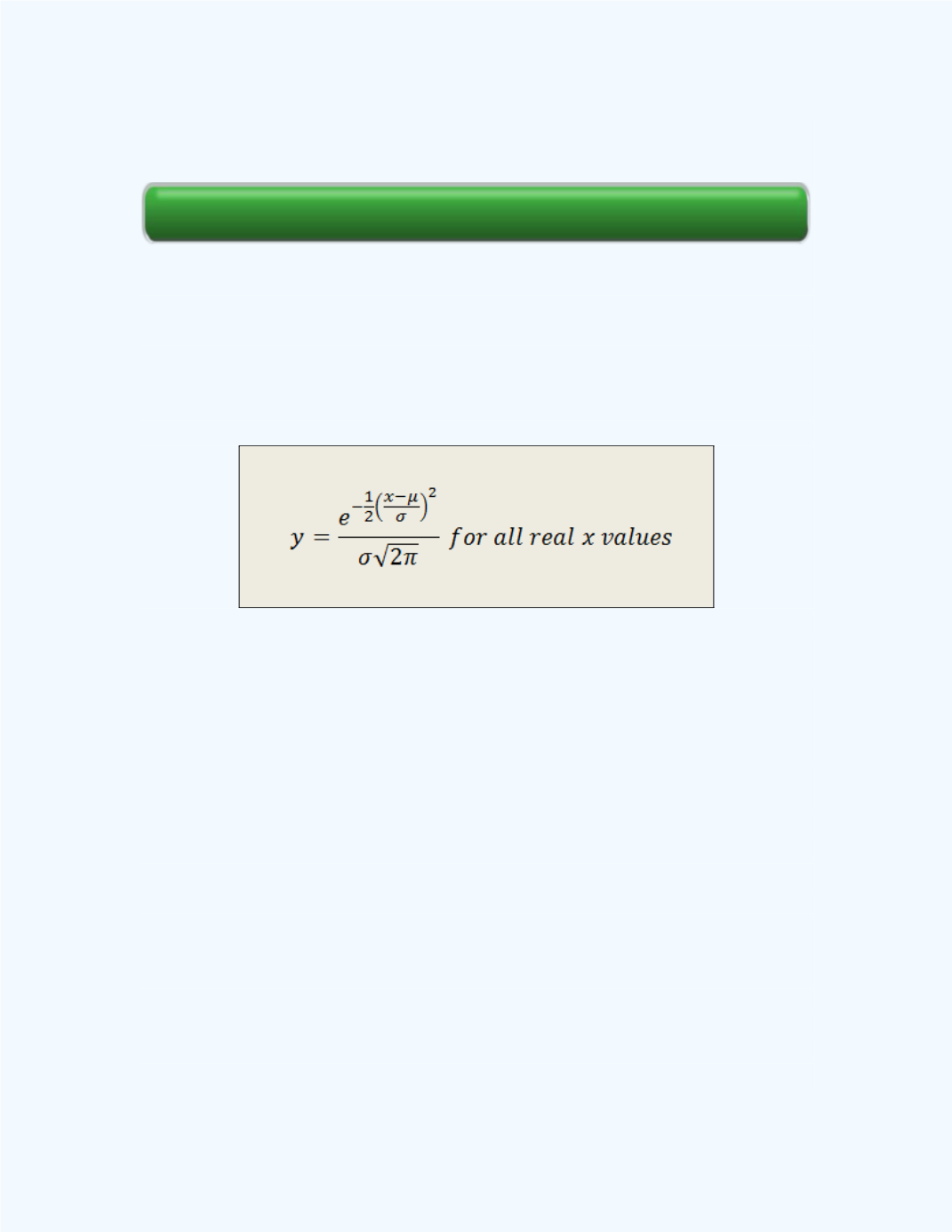
If a random variable
X
is normally distributed, then the mathematical
equation which describes the probability distribution for this random
variable is given by
where,
e
2.718,
3.14,
= population mean, and
= population
standard deviation. The equation says that it true for “
all real x values
”.
This means that the normal variable can assume any value on the real
number line. That is, any value in the interval (-
, +
). When this equation
is graphed for given
and
values, a continuous, bell-shaped, symmetrical
graph will result. Thus, we can display an infinite number of graphs for this
equation, depending on the values of
and
. In such a case, we say we
have a family of normal curves. Because the location and shape of the
distribution depends on the mean
and the standard deviation
, we refer to
these two as the parameters for the distribution. Sometimes we refer to the
mean as the “location” parameter and the standard deviation as the “scale”
parameter. The mean is called the “location” parameter because it tells us
where the origin of the distribution will be located. If the location parameter
is positive, the origin will be shifted to the right and if it is negative the
origin will be shifted to the left. The standard deviation is called the “scale”
parameter because it gives us an idea of the spread of the distribution about
the location parameter. The larger the scale parameter the more spread out
about the location parameter the distribution will be. Some representations
e-Self Review