


 211 / 762

Chapter 5: Bivariate Data
211
Note:
Other forms of the least squares equations for the estimates of
b
0
and
b
1
are possible and may be given by other authors.
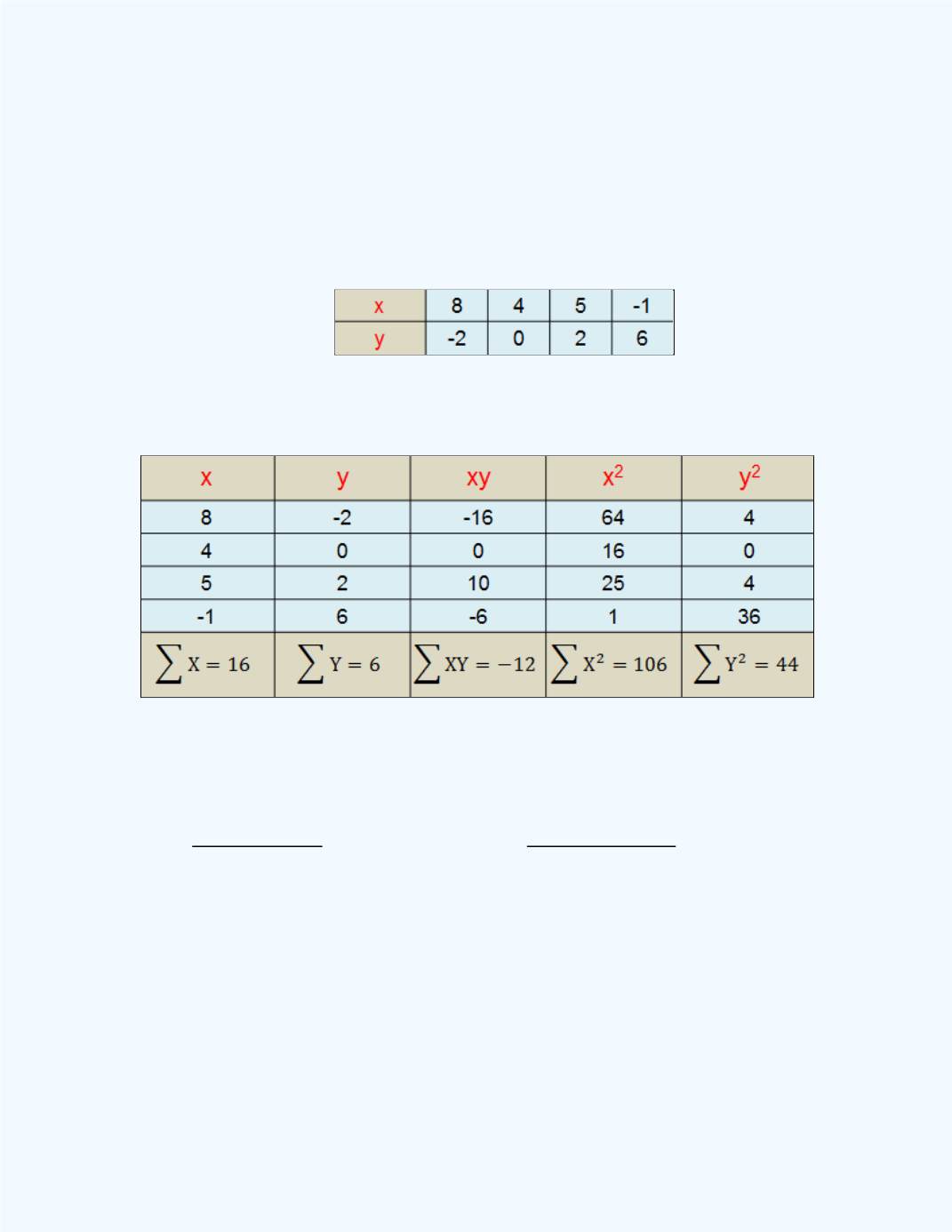
Example 5-3:
Determine the equation for the line of best fit for the
following information where the independent variable is
x
and the dependent
variable is
y
.
Solution:
The formulas for finding b
0
and b
1
may look intimidating, but
we can construct a table, as shown below, to help with the computations.
Thus from the table, we have that
= 4,
∑
,
∑
,
∑
,
and
∑
. Substituting into the formulas for b
0
and b
1
give, to three
decimal places,
( )( ) ( )( )
( ) ( )
, and
( )( ) ( )( )
( ) ( )
Thus, the line of best fit will be given by
̂
+ 4.929. Using the
Simple Regression
workbook, we can display this line of best fit
superimposed on the scatter plot for the data. This is shown in
Figure 5-20
. Observe that the slope of the line is negative which supports
the negative coefficient (the slope) for the
x
term in the model. Observe the
equation for the model is displayed on the graph along with a value for
.
Ignore this value until the discussions found in the next section of the
e-book.