


 214 / 762

214
Chapter 5: Bivariate Data
since the number of cans of soft drinks sold during the day from that
particular vending machine may depend on the recorded daily high
temperature, then one may assume that the quantity will represent the
dependent variable and the daily high temperature will represent the
independent variable. Observe that a vice-versa argument will not be logical
since the daily high temperature could not be dependent on the daily number
of cans of soft drink sold from the machine.
We can use the
Simple Regression
workbook to help with the computation
of the least squares regression equation for the data.
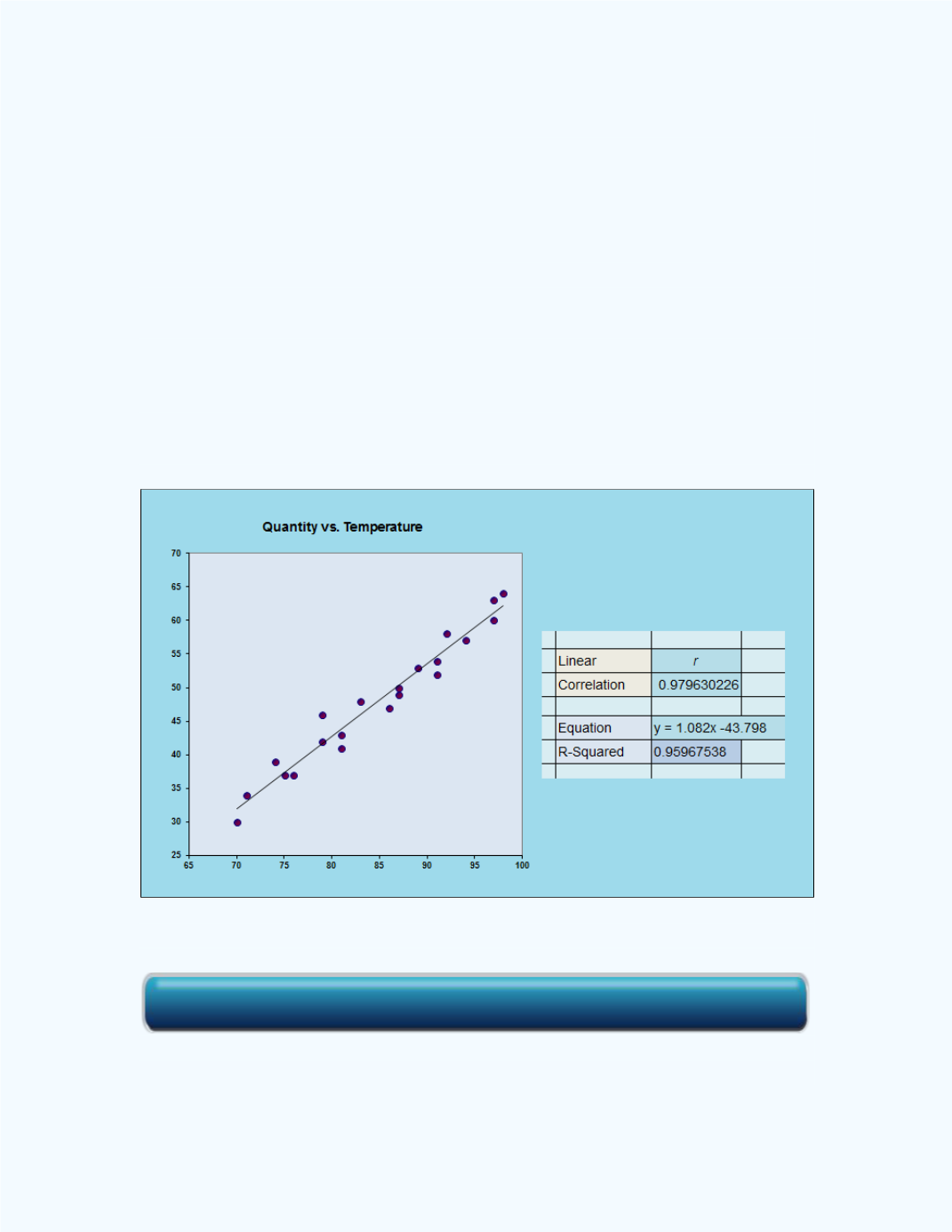
Figure 5-21
displays
the line of best fit superimposed on the scatter plot for the data. Also
included in the figure is the least square regression line or the equation of the
line of best fit. From the equation, the intercept
= -43.798 and the slope
= 1.082. Thus, the line of best fit will be
̂
- 43.798 + 1.082
.
Figure 5-21:
Display of the line of best fit for
Example 5-6
Click here for the Simple Regression Workbook