


 238 / 762

238
Chapter 6: Categorical Data
6-2 Joint and Marginal Distributions
Most of the times in dealing with categorical data, summary tables with the
information are presented. A typical table is usually a cross tabulation of the
respective variables and frequency counts, or relative frequency, or
percentages. One of the things we can create from these summary tables is
called marginal distributions.
In this section, you will be introduced to the concept of joint and marginal
distributions as they apply to contingency tables. You will learn how to
compute the values for both the joint and marginal distributions.
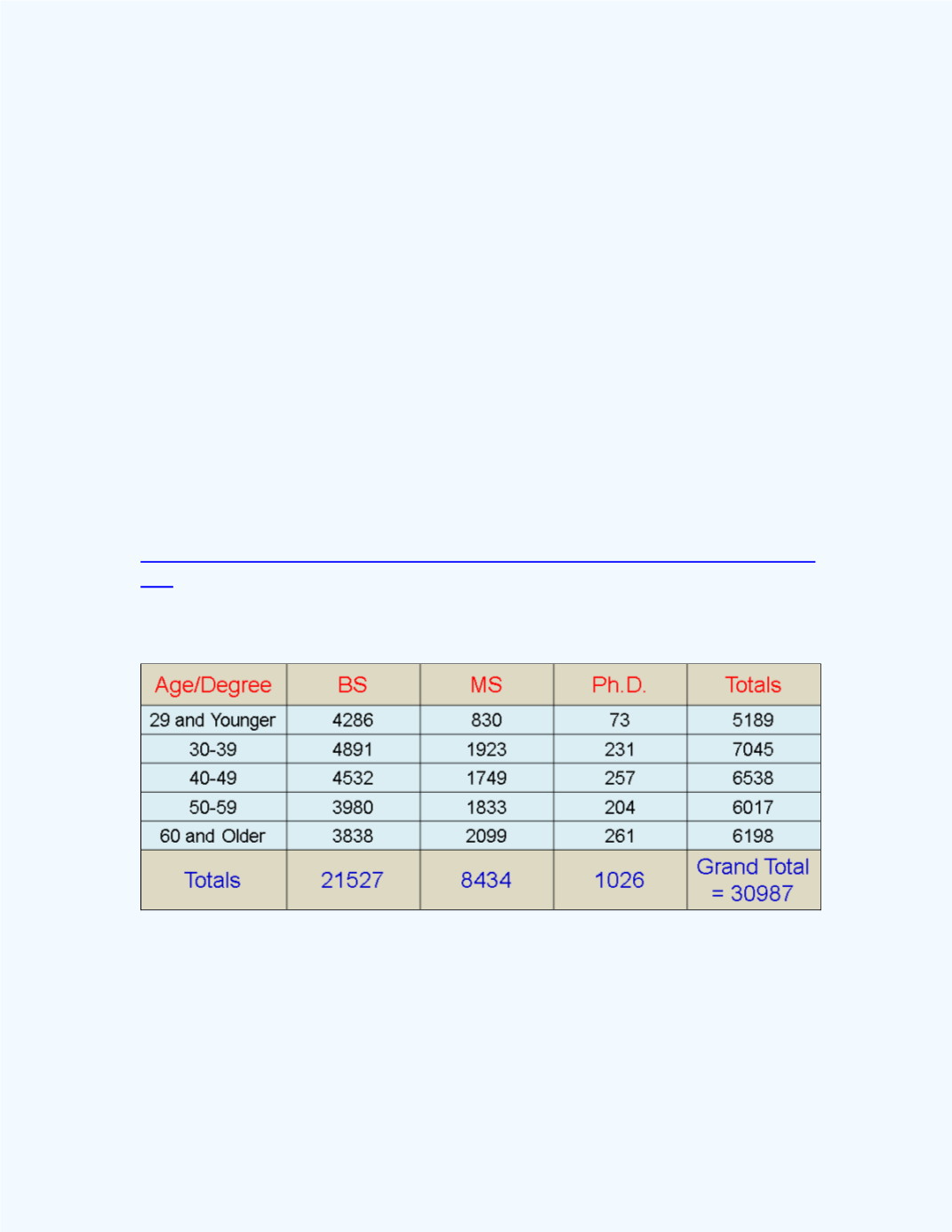
Example 6-1:
A summary of the number of graduates in a BS, MS, and
Ph.D. degree by age (in years) for females 18 years and over from a survey
done in 2010 is given in
Table 1
. Some of the age categories were combined
because of low cell counts and to keep the table to a manageable size.
Source:
http://nces.ed.gov/programs/digest/d10/tables/dt10_009.asp?referrer= list/Table 6-1:
Summary of the Number of Degrees by Age
Table 6-1
represents a two-way contingency table or a bivariate frequency
table since there is only two qualitative variables. This table may sometimes
be called a five by three (5
3) table since we have five classes for the row
(age) classification and three classes for the column (degree) classification.
The table shows how many observations are allocated to each category. Each
row and column combination is called a
cell
in the table. The value of 4,532
in the first column for the degree classification, and the third row for the age