


 447 / 762

Chapter 10: Sampling Distributions and the Central Limit Theorem
447
assumptions hold so we can proceed to invoke the Central Limit Theorem
for the Difference between Two Sample Proportions.
We need to determine
P
(
̂
1
-
̂
2
0.10). We can substitute into
(̂
̂
)
√
to compute the corresponding
-score. That is,
√
= -1.7401. Thus
P
(
̂
1
-
̂
2
0.10) =
P
(
-1.7401)
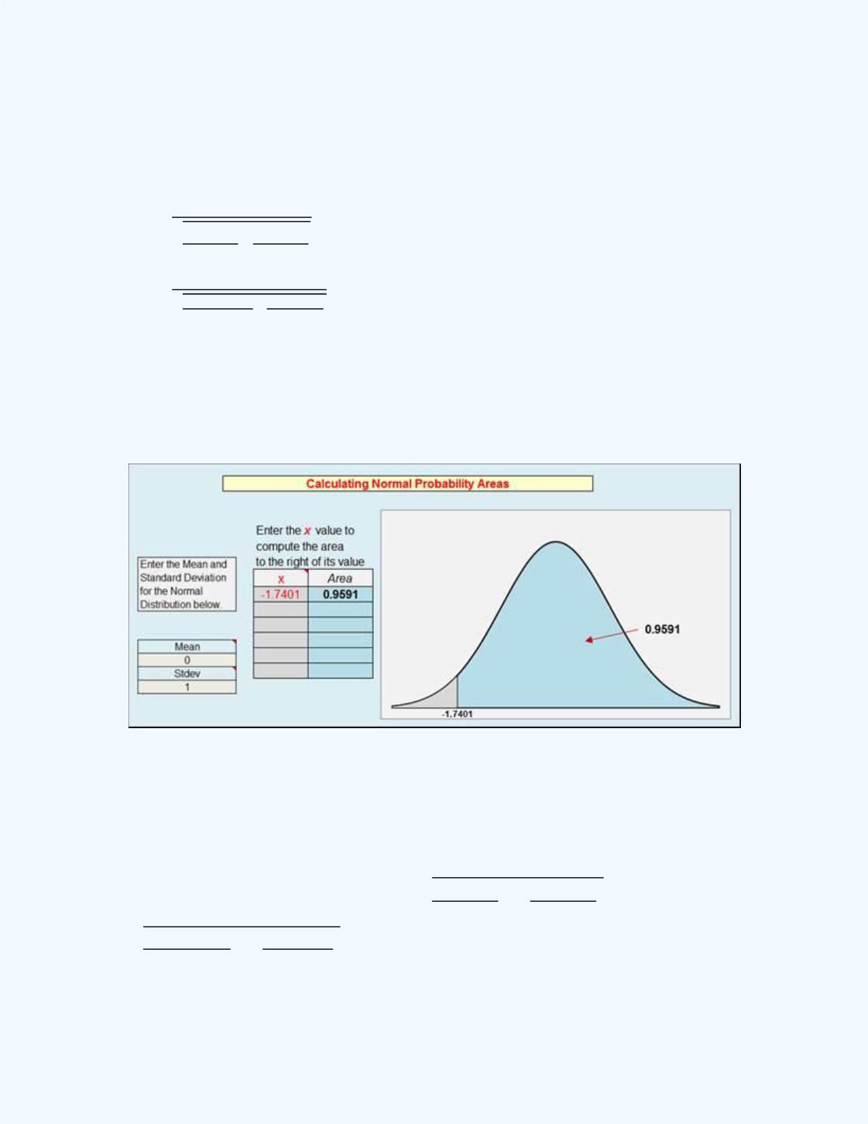
= 0.9591 obtained from the
Normal Probability Distribution
workbook
shown in
Figure 10-23
.
Note:
In the formula for
, you will let
̂
1
-
̂
2
= 0.10 when performing the
computations to evaluate the value of
.
Figure 10-23:
The Normal Distribution output for
P
(z
-1.7401) in
Example 10-5
Also, from the
Central Limit Theorem
, the distribution of
̂
1
-
̂
2
will be
approximately normal with a mean of
̂
̂
= (
p
1
–
p
2
) = 0.75 – 0.5 = 0.25
and a standard deviation of
̂
̂
=
√
=
√
= 0.0862.