


 450 / 762

450
Chapter 10: Sampling Distributions and the Central Limit Theorem
Note:
In the formula for
z
, you will let
̂
1
-
̂
2
= 0.10 and 0.4 when
performing the computations.
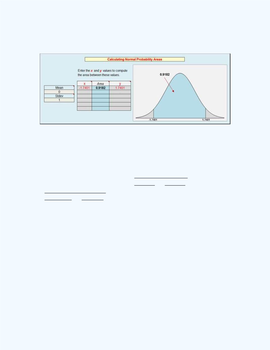
Figure 10-26:
The Normal Distribution Area for
P
(-1.7401
z
1.7401
)
in
Example 10-6
Also, from the
Central Limit Theorem
, the distribution of
̂
1
–
̂
2
will be
approximately normal with a mean of
̂
̂
= (
p
1
–
p
2
) = 0.75 – 0.5 = 0.25
and a standard deviation of
̂
̂
=
√
=
√
= 0.0862.
We can also use these values in the
Normal Probability Distribution
workbook to solve. Use the differences of 0.1 and 0.4. The output is shown
in
Figure 10-27
.